|
The data processing and the construction of 3D magnetic field structure of an active region (AR) is carried out with the extensive use of the IDL program language employing the SolarSoftware general purpose and instrument-specific routines. The SolarSoftware package is a set of integrated software libraries, databases, and system utilities which are suitable for solar common programming and data analysis environment.
For the PF extrapolation as input data, we use hmi.M_45s magnetograms. These are derived every 45 seconds. These provide a full disk image of the line-of-sight (LOS) component of the photospheric magnetic field. These are best used to investigate rapidly evolving field structures (e.g. pre-flare evolution of an AR).
The MONAMI is introduced step by step with a magnetic field observation of AR 11158.
The structure of the MONAMI:
MONAMI /PF:
- 1. Set up the configuration files in the “/PF/configuration/” folder.
- download.ini: “start date” and “end date” of the study period, time-step between the FITS files in seconds.
- parameter.ini: This file for the PF extrapolation. Here, you can set up 1st - maximum box size in km, layer step in km, significance limit of the sunspot contour, limit of sunspot minimum pixel size, all field lines (0) or only closed field lines (1) plot, number of field lines, number of active region.
- 2. To download the hmi.M_45s magnetograms within the given study period ("/PF/configuration/ download.ini"), you can use the "/PF/download_observation.pro" script.
The downloaded FITS files will be in the "/PF/FITS/" folder. ("/PF/FITS/hmi.m_45s.2011.02.15_00_01_30_TAI.magnetogram.fits")
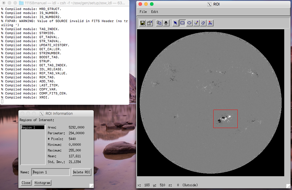
- 3. Cut the interested AR from the full disk images with in the study period by the "/PF/observation_roi.pro". The coordinates of the selected area are stored in the "/PF/configuration/roi.ini" file.
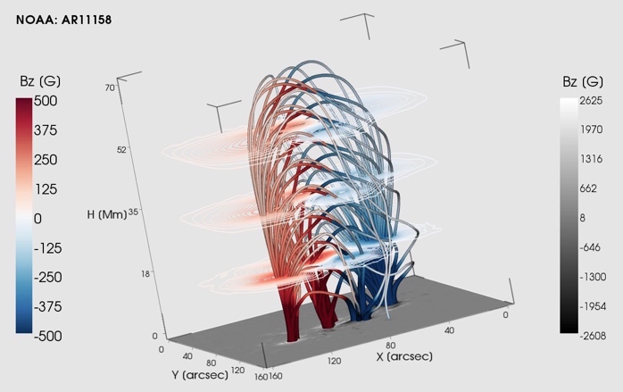
- 4. For the PF extrapolation, you can run the "/PF/extrapolation.pro". This script uses the "/PF/configurat/parameter.ini" file to contract the 3D magnetic field skeleton of the interested AR, what we cut it out from the magnetograms.
The PF extrapolation also use the YAFTA and MPOLE software package. The PF extrapolation itself based on Gary, [ApJ, 69, 323, 1989] and the IDL code was downloaded from here
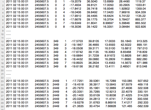
The extrapolation.pro create a catalogue file "/PF/results/results.mp" and an animation file from the extrapolated data.
The "results.mp" data catalogue includes the area, mean magnetic field data and the location (Carrington coordinates, L and B) of sunspots of ARs at every given layer.
MONAMI /PIL:
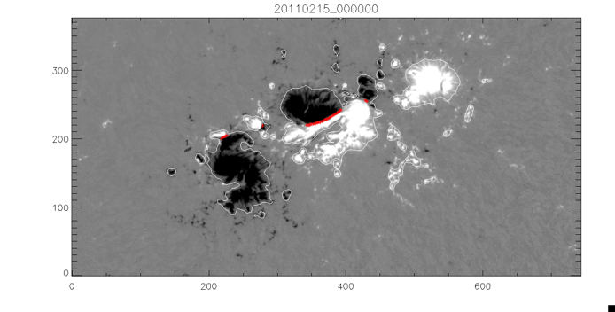
- 5. Apply the automatic PIL recognition program, which was developed by Cui et al. Solar Phys., 237:45–59, 2006.
MONAMI /WG_M:
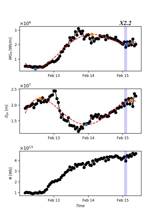
- 6. To calculate the data for WGM-method (Korsós et al. ApJL 2015) run the „/WG_M/osszflux.c “ script, which calculate the unsigned magnetic flux (ϕ), distance (Dpn) and WGM parameters in the identified δ-spot. This program use the results.mp as an input file. The program ask the boundaries of the δ-spot.
- 7. The “/WG_M/polinomfits.py” script is to identified the pre-flare behaviour of the distance (Dpn) and WGM parameters at different height. Set the path and the time intervals.
References:
- G. A. Gary. Linear force-free magnetic fields for solar extrapolation and interpretation. Astrophysical Journal Supplement Series, 69:323–348, 1989
- Y. Cui, R. Li, L. Zhang, Y. He, and H. Wang. Correlation Between Solar Flare Productivity and Photospheric Magnetic Field Properties. 1. Maximum Horizontal Gradient, Length of Neutral Line, Number of Singular Points. Solar Phys., 237:45–59, 2006.
- M. B. Korsós, A. Ludmany, R. Erdélyi, and T. Baranyi. On Flare Predictability Basedon Sunspot Group Evolution. Astrophys. J. Lett.,802:L21, 2015
- Korsós, M. B., Poedts, S., Gyenge, N., Georgoulis, M. K., Yu, S., Bisoi, S. K.,Yan, Y., Ruderman, M. S., Erdélyi, R.: On the evolution of pre-flare patterns of a 3-dimensional model of AR 11429, IAU Conference Series 335, 294-297, 2018
- Korsós, M. B., S. Yang , Erdélyi, R: Pre-flare dynamic investigation by weighted horizontal magnetic gradient method: From small to major flare class, 2019, Journal of Space Weather and Space Climate, 9, id. 12
|